

A Discrete-Time Stochastic Process for Modeling WNBA Career Trajectories
Tackling an often-overlooked front office question through modeling and simulation.


Professional sports are often a “What can you do for me now” business, but championship roster construction often involves years of strategic planning. In this article, I create a framework for forecasting WNBA player careers with front-office decisions in mind. I do this using an approach that both captures the what is of today and projects the what if of tomorrow.
Jump To
Projecting a WNBA Career: Theoretical approach
A player’s career in the WNBA is inherently uncertain. Multi-year forecasts in any field are notoriously tricky, and something as complicated as human growth is especially difficult to model.
For example, take predicting an athlete’s fifth-year stats using only their rookie season. This would be very hard to do, as we aren’t even sure that they’ll still be in the league after four years. What if we take a step back, and pose a much simpler question:
Given a player’s current-season stats, will they retire after this season?
Although this question is a slight abstraction from long-term production, it’s much easier to tackle from a data perspective. Assuming we can build a fairly simple model to answer this first question, we can next address:
Can we quantify potential single-year player progression outcomes?
Again, this is fairly straightforward to answer using the right data. Given that we can (1) predict if a player will retire after the current season and (2) capture potential single-year progression, we can build a robust career-forecasting system. This involves the following:
Create a model to predict retirement, given current-season stats
Apply this model to a player, and determine potential retirement
If a player retires, end their ‘career’
If the player doesn’t retire, apply single-year player progression
Repeat steps 1-4 until a player retires!
You’re probably wondering, how can you reliably predict single-year progression? In this case, I’m not going to try to. Instead, I’ll use background knowledge of similar players to build a range of possible outcomes, and randomly apply one of those outcomes to the player. Then, we can repeat this career simulation many times, giving us a distribution of potential outcomes. With these potential outcomes we can then say:
If a player is in the league in 4 years, here’s what we expect their stats to look like.
One example of this approach (and its application in this article), is forecasting an athlete’s average remaining career length and retirement age:
Modeling WNBA Retirement
To model retirement in the WNBA, I predict if a player will appear in a future season, given their current-season stats. I use logistic regression with 5 inputs: three-point percentage, usage, minutes per game, age, and games played. There’s room for growth in both model and feature selection, but it’s a solid and interpretable starting point.
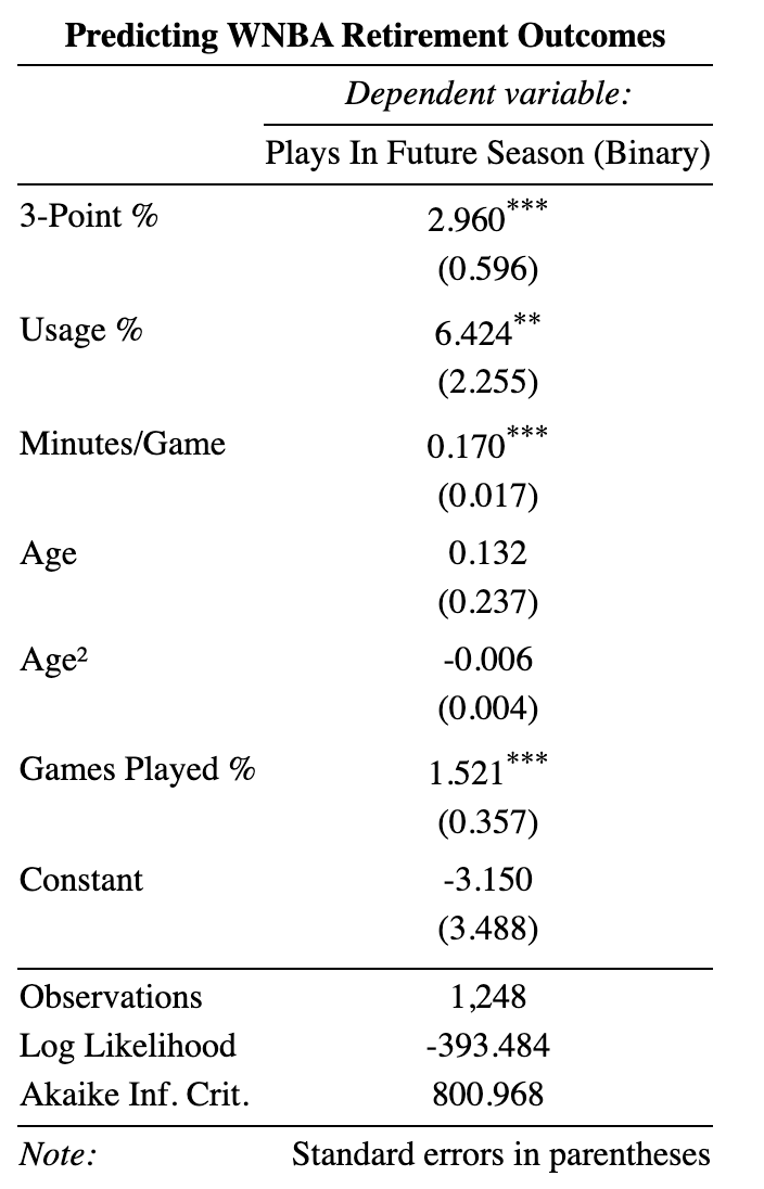
Despite its simplicity, the model is strong, correctly predicting retirement outcomes 85.7% of the time. It excels when predicting continuity (correctly identifying returners 94.8% of the time) and is weaker at predicting retirement (correctly identifying 45.7% of retirements). There’s a bit of a class imbalance at play here, and I’ll add a footnote for how I’m handling it.1
A great example of this model’s strength is applying its predictions out-of-sample to the 2024 season:
Looking at players who were incorrectly predicted as returning in 2025, the top three misses are:
Chennedy Carter (likely due to non-basketball reasons)
Betnijah Laney-Hamilton (season-ending meniscus tear in Unrivaled)
Jordon Horston (season-ending ACL tear in Athletes Unlimited)
Overall, I’m quite pleased with the results. It’s really hard to predict non-basketball situations like the above three without scouting or other input, and I think it’s impressive how such a simple model could offer such strong performance. Now that we have a solid method of predicting retirements, we can continue to forecast player progression.
Simulating Player Progression over Time
To project future progression, I use a discrete-time process, applying changes to players at the end of each simulated year. Potential progression outcomes are created using historical data on similar-aged players. Using this data, players’ stats randomly grow or contract. Over repeated career simulations, this stochastic process gives a distribution of potential outcomes. For example, the chart below shows historical year-over-year changes in minutes per game by age:
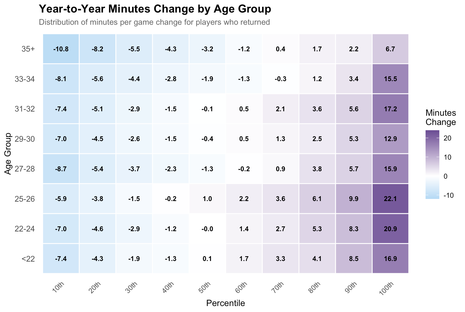
Growth in minutes played can’t exceed a specific cap, and if a player’s projected minutes drop to zero, they retire. Similar caps are applied to the other inputs (usage, games played, three-point percentage). These caps ensure that the range of potential values remains reasonable. They also help correct for the previously-mentioned class imbalance, naturally addressing the first model’s tendency to under-predict retirement.
The Benefits of What-If Analysis & Simulation
I’ll use two examples to demonstrate why combining modeling with simulation is beneficial, the first being Caitlin Clark. Playing just 29% of her team’s games this past season due to injury, she’s forecasted an average remaining career length of only 7 years. Largely due to her limited availability, the most common simulated outcome is just 2 more years. I don’t think this is a true representation of her potential:
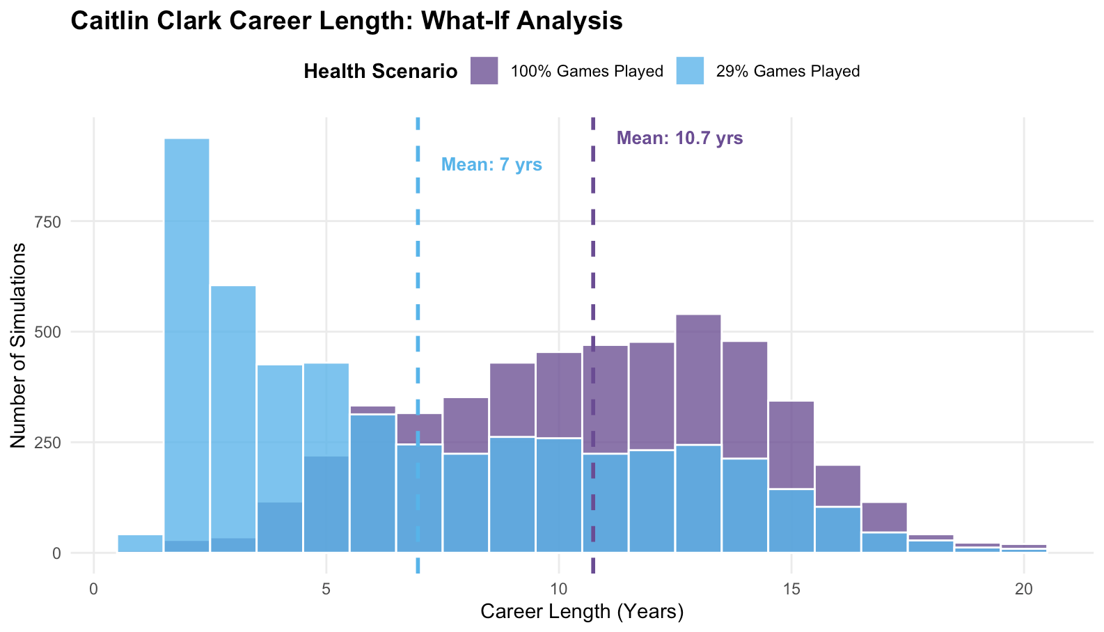
If we gave Caitlin Clark a hypothetical 100% games played last year (which she achieved her rookie season), her projected career length balloons to an average of 10.7 years. With that adjustment, her most-common forecasted outcome becomes a 13-year career. This seems much more realistic and exemplifies how a simple, general model can still be useful for case-by-case analysis. Another way to tackle this idea would be to look at Clark’s career length outcomes conditional on her remaining in the league for at least two more years.
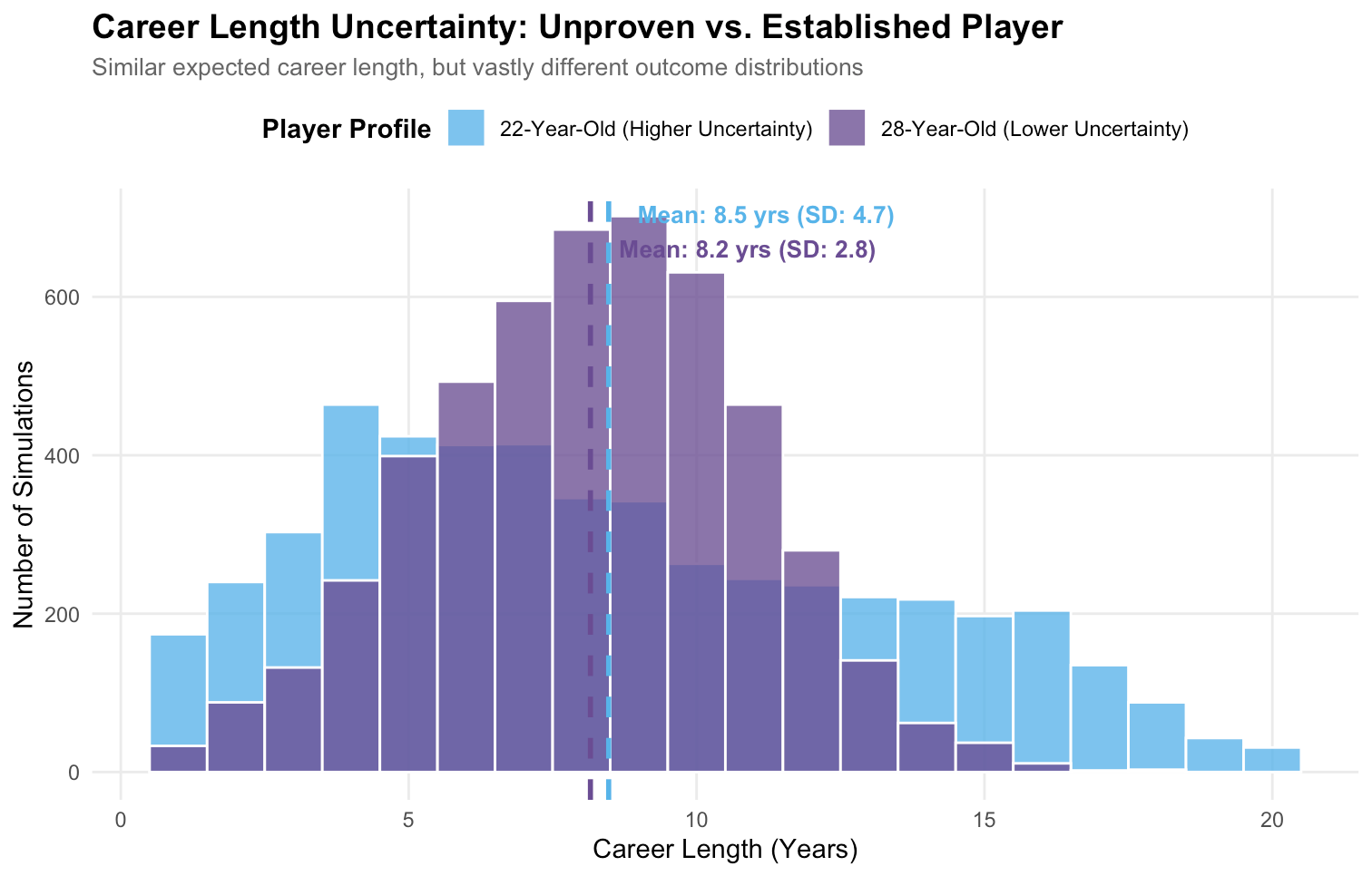
A stochastic process is also great at conveying uncertainty. The above chart compares two players with similar average projected remaining career lengths, but wildly different uncertainty. Jackie Young (purple) is a proven WNBA player who had a much stronger 2025 season. Aziaha James (blue) is a high-upside prospect, and we’re much less certain about what her career could look like. This can be shown through the distribution of potential outcomes: Jackie Young’s interquartile range (IQR) is 4 years, while Aziaha James’ IQR is 7 years.
Applications and Future Improvements
There’s a lot that can be done which I haven’t explicitly discussed in this write-up. For example, here are a couple of questions you could answer using this project:
What does 75th percentile progression look like for two players? Does one have higher upside than the other?
If a player grows their three-point percentage from 35% to 38%, how much does that extend their career in the W?
Will this player still be a ‘bargain’ by the end of their multi-year contract? How likely they are to decline to unplayable in the next three years?
These answers would be pivotal in supporting front-office decision-making, offering an essential data-backed perspective.
From a modeling standpoint, there are many improvements to be made. Instead of using logistic regression, I’d love to use a foundation model such as tabPFN. Second, creating a state-space model would be a clear improvement for forecasting player progression. This would allow progression to account for all stats simultaneously, and also make future progression more dependent on a player’s current state.
Although one of the current strengths is simplicity, I think a true player valuation system would need to consider a few more inputs. As you answer more questions it’d be worth changing the inputs or building a slightly more complex system of models.
To continue the conversation, feel free to leave a comment here on Substack or reach out to me directly on LinkedIn. I appreciate you reading this far and would love your thoughts!
Although there’s a class imbalance affecting this model, there are three reasons why I didn’t apply resampling or weights. First, the cost of errors is asymmetric: falsely predicting retirement could prematurely exclude players from future projections, while over-predicting continued play is a more conservative and correctable approach. Second, I naturally correct for this bias in the model through a future step in this project, which I’ll discuss in Simulating Player Progression. Third, for the sake of this write-up, I want to keep things as simple as possible and allow for future added complexity.