Simulating a Full NBA Game in R Studio

When simulating a game, there are three major components. The first component is the empty stats that are used to make a box score. The second component is the calculations of tendencies that are sent to the Possession function. Then, the possessions are run until the game clock reaches zero (unless overtime is required).

General Game Setup - Empty Box Score and Game Clock:

When each game is initialized, an empty box score is created. This means both teams’ shooting results, field goal percentages, rebounds, and defensive stats are set to zero. For a full box score example, see the “Testing the Simulator’s Accuracy” section. Non-traditional box score stats that are tracked are the number of possessions and number of overtimes. In addition to these stats, the previousResult variable is set to zero, and the game clock is set to 48 minutes. 

Team Tendencies Setup:

The game function takes two parameters: team1 name and team2 name. It uses these parameters to filter the teams of interest from the TeamTotal dataset, and build the following tendencies:

The scaling factor (referred to as score in this write up) is the quotient of offensive rating and defensive ratings in the season that the two teams played, as previously mentioned. Shots attempted and shooting percentages are calculated from per game stats, and the turnover percentage is the average of the offensive and defensive teams’ respective turnover percentage and forced turnover percentage. 

Game Clock and Possessions:

After the empty box score is created and the team tendencies are calculated, the possessions begin! Team 1 and 2 alternate possessions, and the stats returned from the possession function are then recorded in the box score. This process is repeated until the game clock reaches zero, and then the game function returns a dataframe that includes the tracked stats for both teams. If the game clock reaches zero and both teams have the same score, then a five minute overtime period is added. This overtime period repeats until the game clock reaches zero and the teams have different scores, just like in real life.

Testing the Simulator’s Accuracy (Tables followed by Explanations):

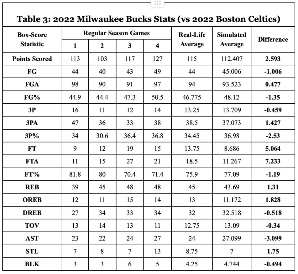
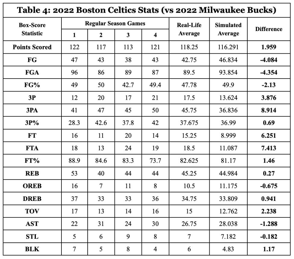
Tables 3 and 4 show the team box score stats from four real-life regular season games, real-life averages of those games, my simulator’s projected averages (from 5,000 simulations), and the difference (real life - simulated) in games played between the 2022 Boston Celtics and 2022 Milwaukee Bucks. All shooting percentages were accurately simulated within 2.5% of the actual average and all box score stats were within 7.5 of the real life average. Table 3 shows the Bucks’ stats and Table 4 shows the Celtics’ stats; they were split up for ease of interpretation but are related to each other in that the two teams were simulated playing against each other.

Overall, I am very satisfied with the simulation accuracy. I ran tests when experimenting between teams from 2016, and then ran validation tests with teams from 2022 once I was satisfied with the 2016 simulation accuracy. The one major difference in real life stats and the model’s projections is that the model predicts many fewer free throws than what actually occurred, and this is because I didn’t include non-shooting fouls (as previously discussed) in my simulations. Additionally, it predicted 8 fewer three pointers attempted for the Celtics than what actually happened, and this may be due to the team’s offensive gameplan. The Buck’s projected three pointers attempted was accurate, so my theory is that the Celtics took more three point shots for one major reason: former MVP Giannis Antetokounmpo clogging the interior of the court forcing the Celtics’ game plan to be very different compared to their usual one, with more outside shots and fewer inside shots attempted. That being said, the Celtics’ three point percentage was still within one  percentage point of what the simulations projected, which I was very satisfied with.